
Please see Part 1 for an introduction to the study that explains how the baskets were determined.
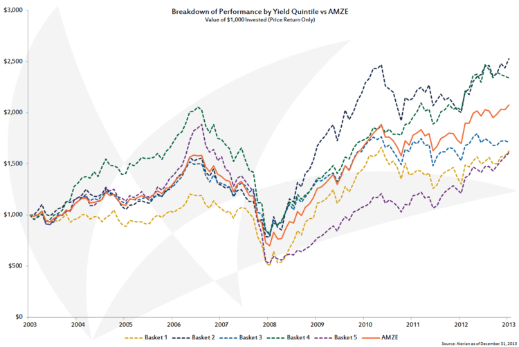
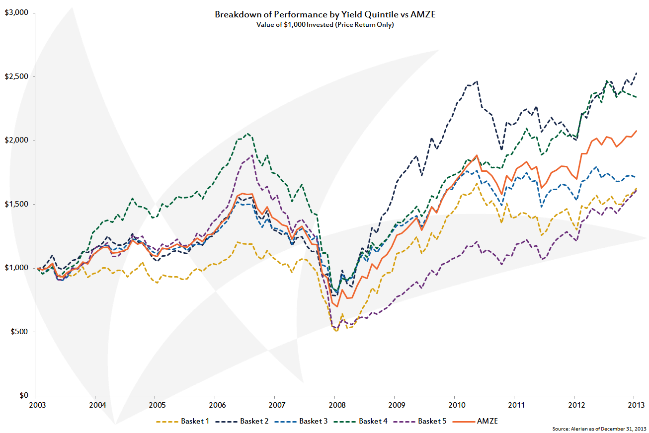
Which quintiles perform the best, and in which markets?
Lower yields may be associated with higher growth, as investors price future distribution increases into current valuation. Lower yields may also be associated with larger companies, which generally own assets across more basins serving different functions along the energy value chain, thereby diversifying risk. With a company of size, however, larger and larger projects must be built (or assets acquired) in order to grow. So, a knee-jerk reaction to buy the lowest-yielding names can lead to underperformance, as evidenced by Basket 5 returning 61% on a price-return basis during the study period as compared to a 108% return for the AMZE.
The middle quintile (Basket 3) also underperformed the index. When a company was acquired or otherwise delisted, it was not replaced until the next annual rebalancing. Basket 3 had four such occurrences during the 10-year period, more than any other basket. Since that security was essentially held static after delisting, it makes sense that Basket 3 would slightly trail the index in a rising market.
Since there’s significant volatility in each quintile, it is worth examining the results on a risk-adjusted basis.
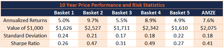
One would assume that the higher-yielding names are more volatile (as measured by standard deviation) than the lower-yielding names. But Basket 5, with the lowest-yielding names and the second-highest standard deviation, suggests that something else is at work. During the financial crisis of 2008, half of the companies in Basket 5 had a negative price return in excess of 75%—more and further than any other basket. Three of the five names were general partners and had leveraged exposure to their underlying MLP. These extreme losses, even in only one year, can influence standard deviation calculations.
The index, with exposure to 50, instead of ten names, has a standard deviation rivaling the least volatile basket. This is one of the benefits of diversified investing—exposure to a broader range of names can often help smooth returns.
Raw measures of risk are useful, but not all risk is rewarded. One way to measure which kinds of risks are worthwhile is to use the Sharpe ratio. Developed by Nobel laureate William Sharpe, the Sharpe ratio subtracts a risk-free rate from the return, with the result divided by the standard deviation. In this way, investors can measure how much of the return, over and above a “safe” return, they are receiving per unit of risk they take on. A Sharpe ratio of zero indicates that the investment would be equivalent to owning the risk-free asset, while a negative ratio indicates that the risk-free asset would outperform. The best risk-adjusted investments are those with the highest Sharpe ratios.
Examining the Sharpe ratios in this study, Baskets 2 and 4 were the sweet spots for MLP investing over the past decade. An investment tracking the AMZE provided a balance of income and growth for investors looking for some exposure to the riskier names.
In part 3, we’ll examine the results on a total-return basis.

